[ 머신러닝 ] 랜덤 포레스트

2023. 9. 11. 17:35ㆍ머신러닝

728x90

1. hotel 데이터셋 알아보기

import matplotlib.pyplot as plt
import numpy as np
import pandas as pd
import seaborn as sns

# csv 파일이 구글드라이브에 있습니다.
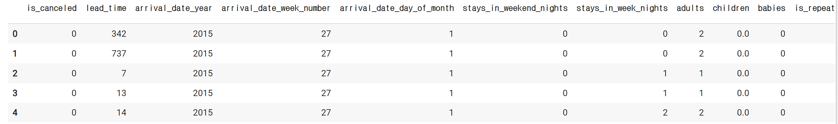
hotel_df = pd.read_csv('/content/drive/MyDrive/Colab Notebooks/9. 머신러닝과 딥러닝/hotel.csv')

hotel_df.head()

# 결과

pd.set_option('display.max_columns', 100)

hotel_df.head()

# 결과

hotel_df.info()

# 결과

# 설명

hotel: 호텔 종류
is_canceled: 취소 여부
lead_time: 예약 시점으로부터 체크인 될 때까지의 기간(얼마나 미리 예약했는지)
arrival_data_year: 예약 연도
arrival_date_month: 예약 월
arrival_date_week: 예약 수
arrival_date_day: 예약 일
stays_in_weekend_nights: 주말을 끼고 얼마나 묵었는지
stays_in_week_nights: 평일을 끼고 얼마나 묵었는지
adults: 성인 인원수
children: 어린이 인원 수
babies: 아기 인원 수
meal: 식사
country: 지역
distribution_channel: 어떤 방식으로 예약했는 지
is_repeated_guest: 예약한적이 있는 고객인지
previous_cancellations: 예약을 취소한 횟수
previous_bookings_not_canceled: 예약을 취소하지 않고 정상 숙박한 횟수
reserved_room_type: 희망 룸 타입
assigned_room_type: 실제 배정된 룸 타입
booking_changes: 예약 후 서비스가 변경된 횟수
deposit_type: 요금 납부 방식
days_in_waiting_list: 예약을 위해 기다린 날짜
customer_type: 고객 타입
adr: 특정일에 높아지거나 낮아지는 가격
required_car_parking_spaces: 주차 공간을 요구했는 지
total_of_special_requests: 특별한 요청사항
reservation_status_date: 예약한 날짜
name: 이름
email: 이메일
phone-number: 휴대폰 번호
credit_card: 카드번호

# df에서 필요한것만 넣기
hotel_df.drop(['credit_card', 'email', 'name', 'phone-number', 'reservation_status_date'], axis=1, inplace=True)

hotel_df.head()

# 결과

hotel_df.describe()
# 아웃라이어 있나 확인

# 결과

 sns.displot(hotel_df['lead_time'])

# 결과

sns.boxplot(y = hotel_df['lead_time'])

# 결과

sns.barplot(x=hotel_df['distribution_channel'], y=hotel_df['is_canceled'])
# undefined 데이터 수 확인 필요

# 결과

hotel_df['distribution_channel'].value_counts()

# 결과

sns.barplot(x=hotel_df['hotel'], y=hotel_df['is_canceled'])

# 결과

sns.barplot(x=hotel_df['arrival_date_year'], y=hotel_df['is_canceled'])

# 결과

plt.figure(figsize=(15,5))
sns.barplot(x=hotel_df['arrival_date_month'], y=hotel_df['is_canceled'])

# 결과

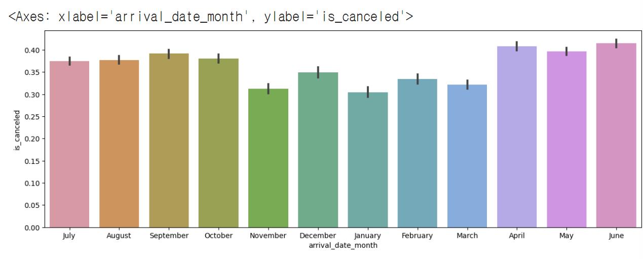
# 월별로 x축을 정렬하기
import calendar

print(calendar.month_name[1])
print(calendar.month_name[2])
print(calendar.month_name[3])

# 결과

months = []

for i in range(1, 13):
  months.append(calendar.month_name[i])
  
months

# 결과

# order로 정렬 가능
plt.figure(figsize=(15,5))
sns.barplot(x=hotel_df['arrival_date_month'], y=hotel_df['is_canceled'], order=months)

# 결과

sns.barplot(x=hotel_df['is_repeated_guest'], y=hotel_df['is_canceled'])
# 처음 온 사람이 취소 확률이 더 높다.

# 결과

sns.barplot(x=hotel_df['deposit_type'], y=hotel_df['is_canceled'])

# 결과

hotel_df['deposit_type'].value_counts()

# 결과

plt.figure(figsize=(15,15))
sns.heatmap(hotel_df.corr(), cmap='coolwarm', vmax=1, vmin=-1, annot=True) # vmin~vmax 이 사이값으로 정규화 시켜라 /  annot=True 네모 박스안에 숫자를 넣어라
# red: 양의 상관관계, blue: 음의 상관관계 -> 색이 진할수록 깊은 관계가 있음

# 결과

hotel_df.isna().mean()

# 결과

hotel_df = hotel_df.dropna()
hotel_df.head()

# 결과

hotel_df[hotel_df['adults']==0]

# 결과

hotel_df['people'] = hotel_df['adults'] + hotel_df['children'] + hotel_df['babies']

# 결과

hotel_df.head()

# 결과

hotel_df[hotel_df['people']==0]

# 결과

hotel_df = hotel_df[hotel_df['people'] != 0]
hotel_df

# 결과

hotel_df['total_nights'] = hotel_df['stays_in_week_nights'] + hotel_df['stays_in_weekend_nights']

# 결과

hotel_df[hotel_df['total_nights'] == 0]

# 결과

hotel_df['arrival_date_month'].apply(lambda x: 'spring' if x in ['March', 'April', 'May'] else 'summer' if x in ['June', 'July', 'August'] else 'fall' if x in ['September', 'October',  'November'] else 'winter')

# 결과

season_dic = {'spring': [3,4,5], 'summer': [6,7,8], 'fall': [9,10,11], 'winter':[12,1,2]}

new_season_dic = {}
for i in season_dic:
  for j in season_dic[i]:
    new_season_dic[calendar.month_name[j]] = i
    
new_season_dic

# 결과

hotel_df['season'] = hotel_df['arrival_date_month'].map(new_season_dic)
hotel_df.head()

# 결과

hotel_df['expected_room_type'] = (hotel_df['reserved_room_type'] == hotel_df['assigned_room_type']).astype(int)
hotel_df.head()

# 결과

hotel_df['cancel_rate'] = hotel_df['previous_cancellations'] / (hotel_df['previous_cancellations'] + hotel_df['previous_bookings_not_canceled'])
hotel_df.head()

# 결과

hotel_df[hotel_df['cancel_rate'].isna()] # NaN이 나온 사람들은 처음 방문한 사람들

# 결과

hotel_df[~hotel_df['cancel_rate'].isna()] # 0.0이라는 건 방문한 적은 있으나 cancel이 없는 경우

# 결과

hotel_df[hotel_df['cancel_rate'] > 0 ] # 캔슬한적이 있는 경우

# 결과

hotel_df['cancel_rate'] = hotel_df['cancel_rate'].fillna(-1)
hotel_df.info()

# 결과

<class 'pandas.core.frame.DataFrame'>
Int64Index: 118728 entries, 0 to 119389
Data columns (total 32 columns):
 #   Column                          Non-Null Count   Dtype  
---  ------                          --------------   -----  
 0   hotel                           118728 non-null  object 
 1   is_canceled                     118728 non-null  int64  
 2   lead_time                       118728 non-null  int64  
 3   arrival_date_year               118728 non-null  int64  
 4   arrival_date_month              118728 non-null  object 
 5   arrival_date_week_number        118728 non-null  int64  
 6   arrival_date_day_of_month       118728 non-null  int64  
 7   stays_in_weekend_nights         118728 non-null  int64  
 8   stays_in_week_nights            118728 non-null  int64  
 9   adults                          118728 non-null  int64  
 10  children                        118728 non-null  float64
 11  babies                          118728 non-null  int64  
 12  meal                            118728 non-null  object 
 13  country                         118728 non-null  object 
 14  distribution_channel            118728 non-null  object 
 15  is_repeated_guest               118728 non-null  int64  
 16  previous_cancellations          118728 non-null  int64  
 17  previous_bookings_not_canceled  118728 non-null  int64  
 18  reserved_room_type              118728 non-null  object 
 19  assigned_room_type              118728 non-null  object 
 20  booking_changes                 118728 non-null  int64  
 21  deposit_type                    118728 non-null  object 
 22  days_in_waiting_list            118728 non-null  int64  
 23  customer_type                   118728 non-null  object 
 24  adr                             118728 non-null  float64
 25  required_car_parking_spaces     118728 non-null  int64  
 26  total_of_special_requests       118728 non-null  int64  
 27  people                          118728 non-null  float64
 28  total_nights                    118728 non-null  int64  
 29  season                          118728 non-null  object 
 30  expected_room_type              118728 non-null  int64  
 31  cancel_rate                     118728 non-null  float64
dtypes: float64(4), int64(18), object(10)
memory usage: 29.9+ MB

hotel_df['country'].dtype # dtype('o') object만 'O'라고 나옴
-------------------------------------------------------------
# 결과
dtype('O')

hotel_df['people'].dtype
-------------------------------
# 결과
dtype('float64')

obj_list = []
for i in hotel_df.columns:
  if hotel_df[i].dtype == 'O':
    obj_list.append(i)
    
obj_list
--------------------------------------
# 결과
['hotel',
 'arrival_date_month',
 'meal',
 'country',
 'distribution_channel',
 'reserved_room_type',
 'assigned_room_type',
 'deposit_type',
 'customer_type',
 'season']

for i in obj_list:
  print(i,hotel_df[i].nunique())
------------------------------------------
# 결과
hotel 2
arrival_date_month 12
meal 5
country 177
distribution_channel 5
reserved_room_type 9
assigned_room_type 11
deposit_type 3
customer_type 4
season 4

hotel_df['meal'].value_counts()
--------------------------------
# 결과
BB           91789
HB           14429
SC           10547
Undefined     1165
FB             798
Name: meal, dtype: int64

hotel_df.drop(['country', 'meal'], axis=1, inplace=True)

obj_list.remove('country')
obj_list.remove('meal')

hotel_df = pd.get_dummies(hotel_df, columns=obj_list)

hotel_df.head()

# 결과

from sklearn.model_selection import train_test_split
X_train, X_test, y_train, y_test = train_test_split(hotel_df.drop('is_canceled', axis=1), hotel_df['is_canceled'], test_size=0.3, random_state=10)

2. 랜덤 포레스트(Random Forest)

Decision Tree는 매우 훌륭한 모델이지만 학습 데이터에 오버피팅하는 경향이 있음(가지치기 같은 방법을 통해 부작용을 최소화 할 수 있지만 부족함)
학습을 통해 구성해 놓은 다수의 나무들(Decision Tree)로부터 분류 결과를 취합해서 결론을 얻는 방식의 모델
Decision Tree 기반의 Bagging 앙상블 모델(두개 이상의 모델을 섞어서 사용하는 경우)
- Bagging은 같은 모델을 섞어서 씀
굉장히 인기있는 모델이며, 사용성이 쉽고 성능도 꾀 우수한 편

2-1. 앙상블(Ensemble) 모델

여러개의 머신러닝 모델을 이용해 최적의 답을 찾아내는 기법

<앙상블 모델의 여러 특징>

보팅(Voting):
- 다른 알고리즘 model을 조합해서 사용
- 모델에 대해 투표로 결과를 도출
배깅(Bagging):
- 같은 알고리즘 내에서 다른 sample 조합을 사용
- 샘플 중복 생성을 통해 결과를 도출(K-Fold처럼 데이터 셋 샘플링(조합)을 다르게 하는 듯..)
부스팅(Boosting):
- 이전 오차를 보완해가면서 가중치를 부여
- 성능이 매우 우수하지만, 잘못된 레이블이나 아웃라이어에 대해 필요 이상으로 민감할 수 있음
스태킹(Stacking):
- 여러 모델을 기반으로 예측된 결과를 통해 meta 모델이 다시한번 예측
- 성능 좋은 모델에 한번 더 학습하여 성능을 극으로 끌어 올릴때 활용하지만, 데이터에 너무 친화적으로되어 과대적합을 유발할 수 있음(특히 데이터셋이 적은 경우)

from sklearn.ensemble import RandomForestClassifier
rf=RandomForestClassifier()
rf.fit(X_train, y_train)

# 결과

pred1 = rf.predict(X_test)
pred1
-------------------------------
# 결과
array([0, 0, 0, ..., 0, 0, 0])

proba1 = rf.predict_proba(X_test)
proba1
----------------------------------
# 결과
array([[0.98, 0.02],
       [1.  , 0.  ],
       [0.71, 0.29],
       ...,
       [1.  , 0.  ],
       [0.97, 0.03],
       [0.93, 0.07]])
       
# 첫번째 테스트 데이터에 대한 예측 결과
proba1[0]
--------------------------------------
# 결과
array([0.98, 0.02])

# 모든 테스트 데이터에 대한 호텔 예약을 취소할 확률만 출력
proba1[:, 1]
-------------------------------------------------------
# 결과
array([0.02, 0.  , 0.29, ..., 0.  , 0.03, 0.07])

3. ROC Curve

이진 분류의 성능을 측정하는 도구
민감도와 특이도로 그려지는 곡선을 의미
FPR(False Positive Rate)
- 특이도. 거짓 양성 비율
- FP / TN + FP
- 실제값은 음성이지만, 양성으로 잘못 분류
TPR(True Positive Rate)
- 민감도. 참인 양성비율
- TP / FN + TP
- 실제로 양성이고 양성으로 잘 분류한 것

4. AUC(Area Under the ROC Curve)

ROC 커브와 직선 사이의 면적을 의미
AUC 값의 범위는 0.5~1이며, 값이 클수록 예측의 정확도가 높음

from sklearn.metrics import accuracy_score, confusion_matrix, classification_report, roc_auc_score
accuracy_score(y_test, pred1) # 예측을 한쪽으로 몰아치지는 않았다는걸 알 수 있음
---------------------------------------------------------------------------------------------------
# 결과
0.8642578399168983

confusion_matrix(y_test, pred1) # 예측을 한쪽으로 몰아치지는 않았다는걸 알 수 있음
-------------------------------------------------------------------------------
# 결과
array([[20816,  1542],
       [ 3293,  9968]])

print(classification_report(y_test, pred1)) # support는 데이터 갯수
------------------------------------------------------------------
# 결과
              precision    recall  f1-score   support

           0       0.86      0.93      0.90     22358
           1       0.87      0.75      0.80     13261

    accuracy                           0.86     35619
   macro avg       0.86      0.84      0.85     35619
weighted avg       0.86      0.86      0.86     35619

roc_auc_score(y_test, proba1[:, 1])
# ROC 곡선 아래 면적을 계산하는 함수
----------------------------------------
# 결과
0.9306581926200015

# 하이퍼파라미터 수정 (max_depth=30을 적용)
rf2 = RandomForestClassifier(max_depth=30, random_state=10)
rf2.fit(X_train, y_train)
proba2 = rf2.predict_proba(X_test)
roc_auc_score(y_test, proba2[:, 1])
# 하이퍼 파라미터 적용 전: 0.9307184561495241
# 하이퍼 파라미터 적용(max_depth=30을 적용) 후: 0.9320285483491656
-----------------------------------------------------------------
# 결과
0.9320285483491656


# 하이퍼파라미터 수정 (max_depth=50을 적용)
rf2 = RandomForestClassifier(max_depth=50, random_state=10)
rf2.fit(X_train, y_train)
proba2 = rf2.predict_proba(X_test)
roc_auc_score(y_test, proba2[:, 1])
# 하이퍼 파라미터 적용 전: 0.9307184561495241
# 하이퍼 파라미터 적용(max_depth=30을 적용) 후: 0.9320285483491656
# 하이퍼 파라미터 적용(max_depth=50을 적용) 후: 0.9303745518246758
----------------------------------------------------------------
0.9303745518246758


# 하이퍼파라미터 수정 (min_samples_split=5 을 적용)
rf2 = RandomForestClassifier(min_samples_split=5, random_state=10)
rf2.fit(X_train, y_train)
proba2 = rf2.predict_proba(X_test)
roc_auc_score(y_test, proba2[:, 1])
# 하이퍼 파라미터 적용 전: 0.9307184561495241
# 하이퍼 파라미터 적용(max_depth=30 을 적용) 후: 0.9320285483491656
# 하이퍼 파라미터 적용(max_depth=50 을 적용) 후: 0.9303745518246758
# 하이퍼 파라미터 적용(min_samples_split=5 을 적용) 후: 0.931436154565479
-----------------------------------------------------------------------
# 결과
0.931436154565479


# 하이퍼파라미터 수정 (min_samples_split=7 을 적용)
rf2 = RandomForestClassifier(min_samples_split=7, random_state=10)
rf2.fit(X_train, y_train)
proba2 = rf2.predict_proba(X_test)
roc_auc_score(y_test, proba2[:, 1])
# 하이퍼 파라미터 적용 전: 0.9307184561495241
# 하이퍼 파라미터 적용(max_depth=30 을 적용) 후: 0.9320285483491656
# 하이퍼 파라미터 적용(max_depth=50 을 적용) 후: 0.9303745518246758
# 하이퍼 파라미터 적용(min_samples_split=5 을 적용) 후: 0.931436154565479
# 하이퍼 파라미터 적용(min_samples_split=7 을 적용) 후: 0.9312578210627522
------------------------------------------------------------------------
# 결과
0.9312578210627522


# 하이퍼파라미터 속성이 개별적으로 높다해도, 콜라보했을 때 좋다라는 보장이 없다.
# 하이퍼파라미터에 넣는 값을 알고리즘을 공부하면서 중요 속성 및 그 범위값은 알 필요가 있다.

5. 하이퍼 파라미터 최적의 값을 찾는 방법

GridSearchCV: 원하는 모든 하이퍼 파라미터를 적용하여 최적의 값을 찾아주는 방법

from sklearn.model_selection import GridSearchCV
params = {
    'max_depth': [None, 10, 30, 50],
    'min_samples_split': [2, 3, 5, 7, 10]
}
rf3 = RandomForestClassifier(random_state=10)
grid_df = GridSearchCV(rf3, params, cv=5) # cv: 데이터 교차검증
grid_df.fit(X_train, y_train)

# 결과

grid_df.best_params_
# params 중에서 최고의 하이퍼파라미터 조건을 보여줌
---------------------------------------------------
# 결과
{'max_depth': 30, 'min_samples_split': 2}


rf3 = RandomForestClassifier(max_depth=30, min_samples_split=2, random_state=10)
rf3.fit(X_train, y_train)
proba2 = rf3.predict_proba(X_test)
roc_auc_score(y_test, proba2[:, 1])
# 하이퍼 파라미터 적용(max_depth=30 을 적용, min_samples_split=5 을 적용) 후: 0.9320878540030826
# 최적의 하이퍼 파라미터 값 적용(max_depth=30 을 적용, min_samples_split=2 를 적용) 후: 0.9320285483491656
#  cv: 데이터 교차검증을 넣었기 떄문에, 런타임 다시 실행 시 이 최적의 값 적용한 결과가 더 안좋게 나왔을수도...
-------------------------------------------------------------------------------------------------------
# 결과
0.9320285483491656

6. 피쳐 중요도(Feature Importances)

Decision Tree 에서 노드를 분기할 때 해당 피쳐가 클래스를 나누는데 얼마나 영향을 미쳤는지 표기하는 척도
0이면 클래스를 구분하는데 해당 피쳐가 선택되지 않았다는 것이며, 1이면 해당 피쳐가 클래스를 완벽하게 나눴다는 것을 의미

proba3 = rf3.predict_proba(X_test)
proba3
---------------------------------------
# 결과
array([[0.96333333, 0.03666667],
       [0.98747831, 0.01252169],
       [0.67944316, 0.32055684],
       ...,
       [1.        , 0.        ],
       [0.90383261, 0.09616739],
       [0.97      , 0.03      ]])
       

roc_auc_score(y_test, proba3[:, 1])
-------------------------------------
# 결과
0.9320285483491656

rf3.feature_importances_
-----------------------------------------------------------------------
# 결과
array([1.27137138e-01, 2.14563953e-02, 4.68663037e-02, 5.96305446e-02,
       2.16746957e-02, 3.25152451e-02, 1.02347526e-02, 5.40307416e-03,
       8.84445875e-04, 2.02141842e-03, 2.44460558e-02, 3.14871409e-03,
       2.18776128e-02, 3.06142123e-03, 9.51803193e-02, 2.23244236e-02,
       5.75968205e-02, 1.36759899e-02, 3.53588232e-02, 2.80447856e-02,
       3.80039740e-02, 7.62870375e-03, 6.72543460e-03, 3.44290597e-03,
       4.03857944e-03, 2.04861894e-03, 2.63415501e-03, 1.84105707e-03,
       3.95932072e-03, 3.62772728e-03, 3.05844877e-03, 3.56107858e-03,
       2.38180451e-03, 3.26791942e-03, 2.91845948e-03, 3.01678974e-03,
       9.42477811e-03, 2.46969262e-04, 1.08307976e-02, 0.00000000e+00,
       5.74350945e-03, 9.03907596e-04, 6.54901146e-04, 4.05826969e-03,
       2.30412987e-03, 1.25861929e-03, 1.10018824e-03, 3.65382816e-04,
       3.43650984e-05, 1.10160554e-02, 1.51175712e-03, 1.19112472e-03,
       5.19366703e-03, 2.61859311e-03, 1.46746839e-03, 1.15967758e-03,
       3.98805744e-04, 1.35937049e-04, 1.43906056e-04, 2.28125116e-06,
       6.99747351e-02, 9.55569434e-02, 4.52910589e-04, 3.08796348e-03,
       4.79153629e-04, 1.67417487e-02, 1.19682713e-02, 3.45258733e-03,
       4.02311808e-03, 4.35533780e-03, 3.44818237e-03])

1.27137138e-01 # 전체 중요도중에서 1.2% 정도의 가중치. 0에 가까울수록 필요없는 feature다.
------------------------------------------------------------------------------------
# 결과
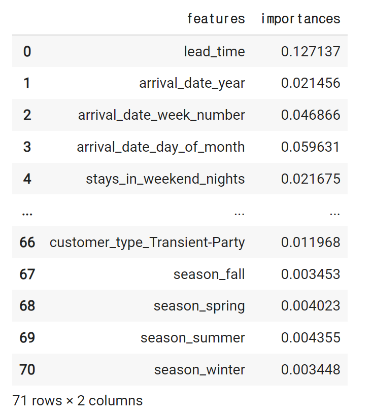
0.127137138

feat_imp = pd.DataFrame({
    'features': X_train.columns,
    'importances': rf3.feature_importances_
})

feat_imp

# 결과

top10 = feat_imp.sort_values('importances', ascending=False).head(10)
top10

# 결과

plt.figure(figsize=(5,10))
sns.barplot(x='importances', y='features', data=top10)

# 결과

728x90

'머신러닝' 카테고리의 다른 글

[ 머신러닝 ] KMEans (0)	2023.09.11
[ 머신러닝 ] lightGBM (0)	2023.09.11
[ 머신러닝 ] 서포트 벡터 머신 (0)	2023.09.06
[ 머신러닝 ] 로지스틱 회귀 (0)	2023.09.06
[ 머신러닝 ] 의사결정나무 (0)	2023.09.06

고예진은 개발과 보이지 않는(애덤스미스 아님) 전쟁중

고예진은 개발과 보이지 않는(애덤스미스 아님) 전쟁중

태그

최근글

댓글

공지사항

아카이브

1. hotel 데이터셋 알아보기

2. 랜덤 포레스트(Random Forest)

2-1. 앙상블(Ensemble) 모델

3. ROC Curve

4. AUC(Area Under the ROC Curve)

5. 하이퍼 파라미터 최적의 값을 찾는 방법

6. 피쳐 중요도(Feature Importances)

'머신러닝' 카테고리의 다른 글

관련글

티스토리툴바