[ 머신러닝 ] 선형회귀
2023. 9. 6. 02:10ㆍ머신러닝
728x90
🌀 Rent 데이터셋 살펴보기
import numpy as np
import pandas as pd
import seaborn as sns
# rent.csv 파일이 이미 있는 상태에요!
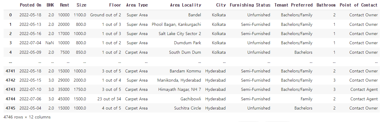
rent_df = pd.read_csv( '/content/drive/MyDrive/머신러닝 딥러닝/rent.csv')
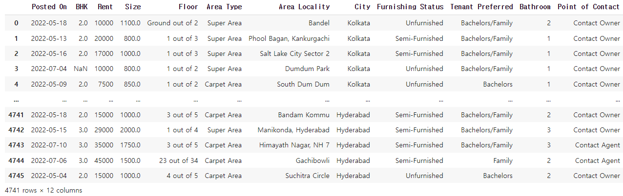
rent_df✔️ 결과
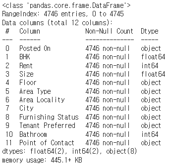
rent_df.info()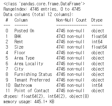
rent_df.info() 결과의 부가설명
* Posted On: 매물 등록 날짜
* BHK: bed, hall, kitchen 개수
* Rent: 렌트비
* Size: 집 크기
* Floor: 총 층수 중 몇 층인지
* Area Type: 공용공간을 포함하는지, 집의 면적만 포함하는지
* Area Locality: 지역
* City: 도시
* Furnishing Status: 가구 옵션 여부
* Tenant Preferred: 선호하는 가족 형태
* Bathroom: 화장실 개수
* Point of Contact: 연락할 곳
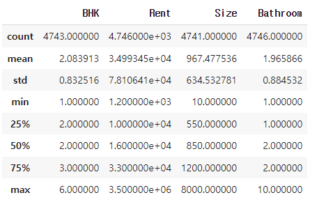
# describe() 함수는 수치 기준으로 나온 데이터들을 테이블로 변환
rent_df.describe()
✔️결과
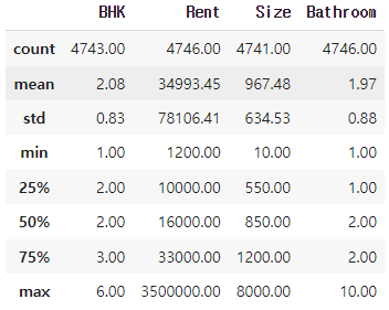
# 소수 뒤 두자리까지만 표시
round(rent_df.describe(), 2)
✔️결과
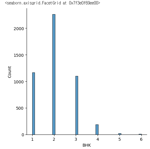
sns.displot(rent_df['BHK'])✔️ 결과
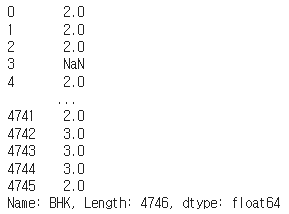
rent_df['BHK']✔️ 결과
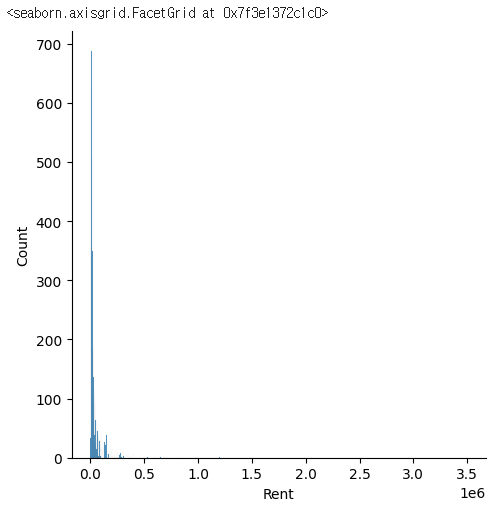
sns.displot(rent_df['Rent'])✔️ 결과
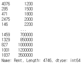
rent_df['Rent'].sort_values()✔️ 결과
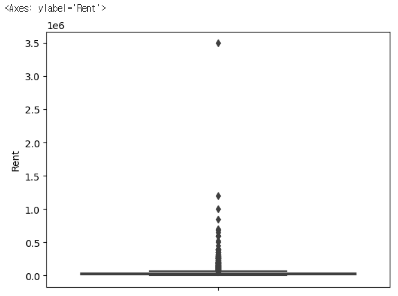
sns.boxplot(y=rent_df['Rent'])✔️ 결과
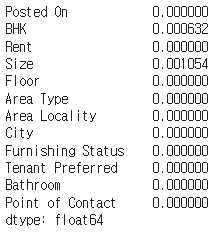
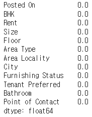
rent_df.isna().mean()✔️ 결과
# Size에 있는 결측치 데이터를 삭제
rent_df.dropna(subset=['Size'])
✔️ 결과
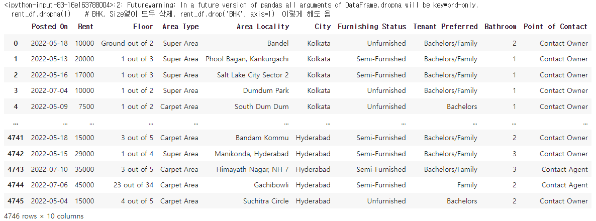
# 결측치가 있는 열을 삭제. 1이 열을 의미함
rent_df.dropna(1)    # BHK, Size열이 모두 삭제. rent_df.drop('BHK', axis=1)  이렇게 해도 됨
✔️ 결과
# rent_df 데이터프레임에서 Size 컬럼이 NaN 인 행을 모두 출력
rent_df[rent_df['Size'].isna()]
✔️ 결과
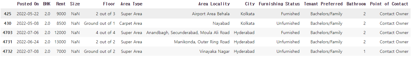
na_index = rent_df[rent_df['Size'].isna()].index
na_index
--------------------------------------------------
# 결과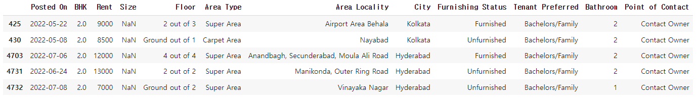
Int64Index([425, 430, 4703, 4731, 4732], dtype='int64')rent_df.iloc[na_index]✔️ 결과
# 결측치 처리
# 1. 결측 데이터가 전체 데이터에 비해 양이 굉장히 적을 경우 삭제하는 것도 방법
# 2. 결측치에 데이터를 채울 경우 먼저 boxplot을 확인하는 것이 좋음
sns.boxplot(y=rent_df['Size'])
✔️ 결과
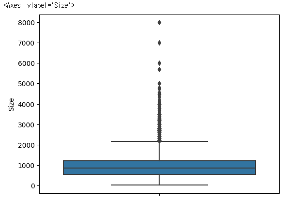
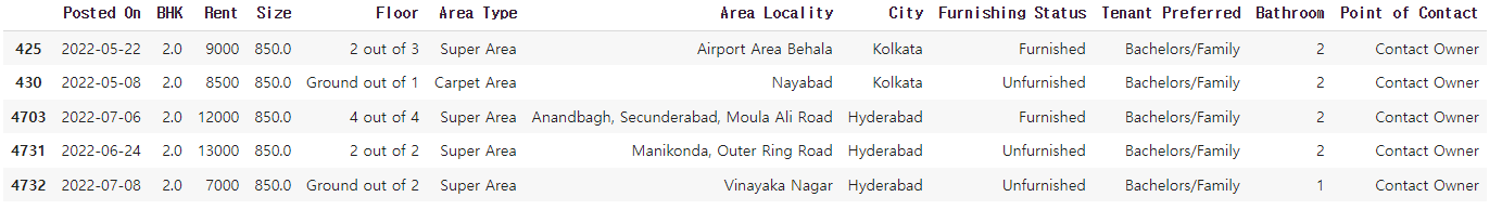
# boxplot을 확인 후 mean 보다는 median을 사용하는게 좋다고 판단!
rent_df.fillna(rent_df.median()).loc[na_index]
✔️결과
na_index = rent_df[rent_df['BHK'].isna()].index
na_index
----------------------------------------------------
# 결과
Int64Index([3, 53, 89], dtype='int64')

rent_df['BHK'].fillna(rent_df['BHK'].median()).loc[na_index]
------------------------------------------------------------
# 결과
3     2.0
53    2.0
89    2.0
Name: BHK, dtype: float64

rent_df = rent_df.fillna(rent_df.median())
-------------------------------------------------------------
# 결과
<ipython-input-91-3059977004fc>:1: FutureWarning: The default value of numeric_only in DataFrame.median is deprecated. In a future version, it will default to False. In addition, specifying 'numeric_only=None' is deprecated. Select only valid columns or specify the value of numeric_only to silence this warning.
rent_df = rent_df.fillna(rent_df.median())rent_df.isna().mean()✔️ 결과
rent_df.info()✔️ 결과
# Area Type은 텍스트 형태이기 때문에 모델에서 계산을 할 수 없음
# 라벨 인코딩을 통해 숫자로 변경
rent_df['Area Type'].value_counts()
-----------------------------------------------------------
# 결과
Super Area     2446
Carpet Area    2298
Built Area        2
Name: Area Type, dtype: int64
rent_df['Area Type'].unique()
---------------------------------------------------------------
# 결과
array(['Super Area', 'Carpet Area', 'Built Area'], dtype=object)
# 유니크한 종류의 개수
rent_df['Area Type'].nunique()
-----------------------------------
# 결과
3
for i in ['Floor', 'Area Type', 'Area Locality', 'City', 'Furnishing Status', 'Tenant Preferred', 'Point of Contact']:
print(i, rent_df[i].nunique())
-----------------------------------------------------------------------------------------------------------------------
# 결과
Floor 480
Area Type 3
Area Locality 2235
City 6
Furnishing Status 3
Tenant Preferred 3
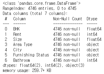
Point of Contact 3rent_df.drop(['Posted On', 'Floor', 'Area Locality', 'Tenant Preferred', 'Point of Contact'], axis=1, inplace=True)rent_df.info()✔️ 결과
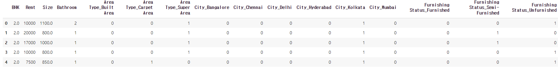
rent_df = pd.get_dummies(rent_df, columns = [ 'Area Type', 'City', 'Furnishing Status'])
rent_df.head()
✔️ 결과
X = rent_df.drop('Rent', axis=1)  # 독립변수
y = rent_df['Rent'] # 종속변수

from sklearn.model_selection import train_test_split

X_train, X_test, y_train, y_test = train_test_split(X, y, test_size=0.2, random_state=10)
X_train.shape, y_train.shape
-----------------------------------------------------------------------------------------
# 결과
((3796, 15), (3796,))

X_test.shape, y_test.shape
------------------------------
# 결과
((950, 15), (950,))
🌀 선형회귀(Linear Regression)
* 데이터를 통해 가장 잘 설명할 수 있는 직선으로 데이터를 분석하는 방법
* 단순 선형 회귀 분석( 단일 독립변수를 이용 )
* 다중 선형 회귀 분석( 다중 독립변수를 이용 )
from sklearn.linear_model import LinearRegression
lr = LinearRegression()
lr.fit(X_train, y_train)
✔️ 결과
🌀 MSE( Mean Squared Error)
- 예측값과 실제값의 차이에 대한 제곱에 대해 평균을 낸 값
- (1n)∑ni=1(yi−xi)2
p = np.array([3,4,5]) # 예측값
act = np.array([1,2,3])  # 실제값

def my_mse(pred, actual):
    return((pred - actual) ** 2).mean()

my_mse(p, act)
------------------------------------------
# 결과
4.0
🌀 MAE( Mean Absolute Error)
- 예측값과 실제값의 차이에 대한 절대값에 대해 평균을 낸 값
- (1n)∑ni=1|yi−xi|
def my_mae(pred, actual):
    return np.abs(pred - actual).mean()
my_mae(p, act)
--------------------------------------------
# 결과
2.0
🌀 RMSE( Root Mean Squared Error)
- 예측값과 실제값의 차이에 대한 제곱에 대해 평균을 낸 후 루트를 씌운 값
- (1n)∑ni=1(yi−xi)2−−−−−−−−−−−−−−−√
def my_rmse(pred, actual):
    return np.sqrt(my_mse(pred, actual))
my_rmse(p, act)
-----------------------------------------
# 결과
2.0

from sklearn.metrics import mean_absolute_error, mean_squared_error
mean_absolute_error(p, act)
---------------------------------------------------------------------
# 결과
2.0

mean_squared_error(p, act)
-----------------------------
# 결과
4.0

mean_squared_error(p, act, squared=False) # RMSE
-------------------------------------------------
# 결과
2.0
🌀 평가지표 적용하기
mean_squared_error(y_test, pred)
-----------------------------------
# 결과
1717185779.0021067

mean_absolute_error(y_test, pred)
-----------------------------------
# 결과
22779.17722543894

mean_squared_error(y_test, pred, squared=False)
------------------------------------------------
# 결과
41438.9403701652
X_train.drop(1837, inplace=True)
y_train.drop(1837, inplace=True)
lr.fit(X_train, y_train)✔️ 결과
pred= lr.predict(X_test)
mean_squared_error(y_test, pred, squared=False)
-------------------------------------------------
# 결과
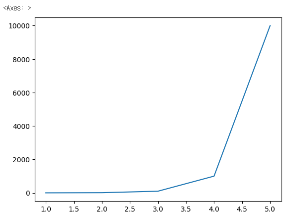
41377.57030234839🌀 log 활용하기
a= [1,2,3,4,5]
b=[1,10,100,1000,10000]

sns.lineplot(x=a, y=b)
✔️ 결과
b_log = np.log(b)
b_log
---------------------------------------------------------------------
# 결과
array([0.        , 2.30258509, 4.60517019, 6.90775528, 9.21034037])

np.exp(b_log)
------------------------------------------------
# 결과
array([1.e+00, 1.e+01, 1.e+02, 1.e+03, 1.e+04])

y_train_log = np.log(y_train)
lr.fit(X_train, y_train_log)
✔️ 결과
728x90
반응형
'머신러닝' 카테고리의 다른 글
| [ 머신러닝 ] 로지스틱 회귀 (0) | 2023.09.06 |
|---|---|
| [ 머신러닝 ] 의사결정나무 (0) | 2023.09.06 |
| [머신러닝] Titanic Dataset (2) | 2023.08.30 |
| [ 머신러닝 ] 아이리스 데이터셋 (0) | 2023.06.25 |
| [ 머신러닝 ] 사이킷런 & Linear SVC (0) | 2023.06.25 |