머신러닝
[ 머신러닝 ] 의사결정나무
예진또이(애덤스미스 아님)
2023. 9. 6. 03:06
728x90
🌀bike 데이터셋 살펴보기
import numpy as np
import pandas as pd
import seaborn as sns
import matplotlib.pyplot as plt
bike_df = pd.read_csv('/content/drive/MyDrive/머신러닝 딥러닝/bike.csv')
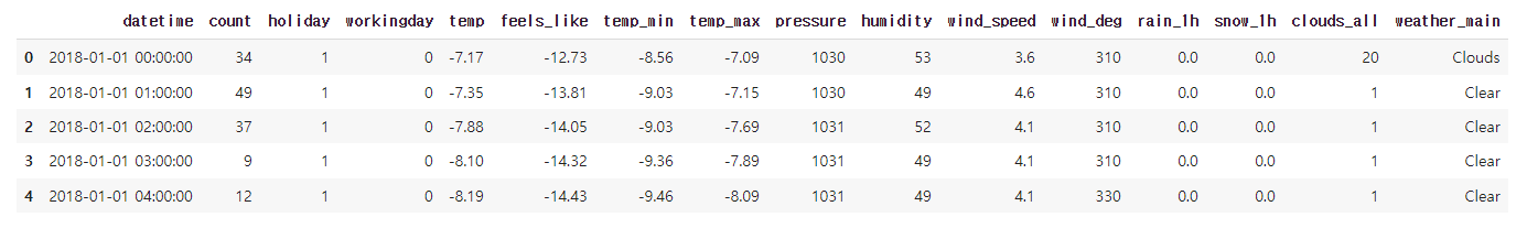
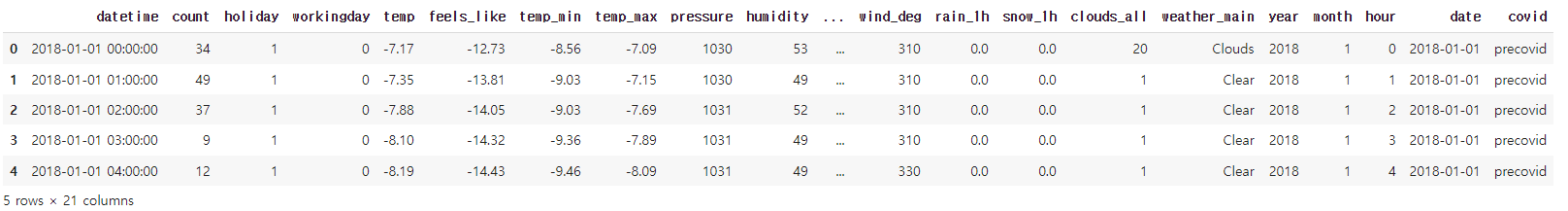
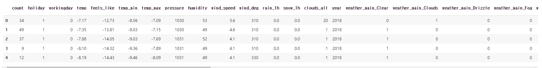
bike_df✔️ 결과
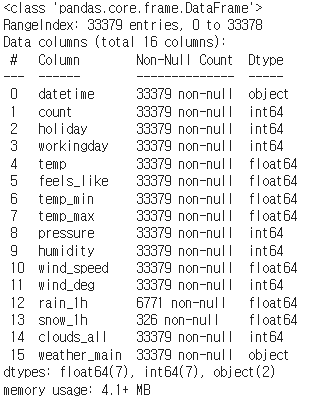
bike_df.info()✔️ 결과
- datetime: 날짜
- count: 대여갯수
- holiday: 휴일
- workingday: 근무일
- temp: 기온
- feels_like: 체감온도
- temp_min: 최저온도
- temp_max: 최고온도
- pressure: 기압
- humidity: 습도
- wind_speed: 풍속
- wind_deg: 풍향
- rain_1h: 강우량
- snow_1h: 강설량
- clouds_all: 구름의 양
- weather_main: 날씨
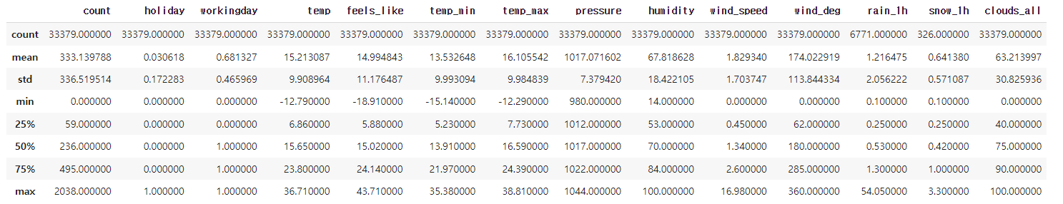
bike_df.describe()✔️ 결과
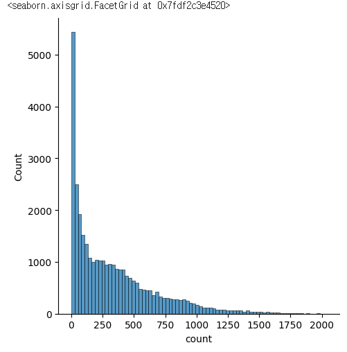
sns.displot(bike_df['count'])
✔️ 결과
sns.boxplot(bike_df['count'])
✔️ 결과

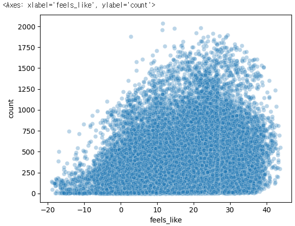
sns.scatterplot(x='feels_like', y='count', data=bike_df, alpha= 0.3)✔️ 결과
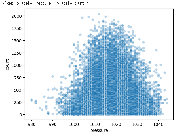
sns.scatterplot(x='pressure', y='count', data=bike_df, alpha=0.3)
✔️ 결과
sns.scatterplot(x='wind_speed', y='count', data=bike_df, alpha=0.3)
✔️ 결과

sns.scatterplot(x='wind_deg', y='count', data=bike_df, alpha=0.3)✔️ 결과

bike_df.isna().sum()
✔️ 결과
datetime            0
count               0
holiday             0
workingday          0
temp                0
feels_like          0
temp_min            0
temp_max            0
pressure            0
humidity            0
wind_speed          0
wind_deg            0
rain_1h         26608
snow_1h         33053
clouds_all          0
weather_main        0
dtype: int64bike_df.isna().mean()✔️ 결과
datetime        0.000000
count           0.000000
holiday         0.000000
workingday      0.000000
temp            0.000000
feels_like      0.000000
temp_min        0.000000
temp_max        0.000000
pressure        0.000000
humidity        0.000000
wind_speed      0.000000
wind_deg        0.000000
rain_1h         0.797148
snow_1h         0.990233
clouds_all      0.000000
weather_main    0.000000
dtype: float64
bike_df = bike_df.fillna(0)
bike_df.isna().mean()
✔️ 결과
datetime        0.0
count           0.0
holiday         0.0
workingday      0.0
temp            0.0
feels_like      0.0
temp_min        0.0
temp_max        0.0
pressure        0.0
humidity        0.0
wind_speed      0.0
wind_deg        0.0
rain_1h         0.0
snow_1h         0.0
clouds_all      0.0
weather_main    0.0
dtype: float64
bike_df.info()
✔️ 결과
<class 'pandas.core.frame.DataFrame'>
RangeIndex: 33379 entries, 0 to 33378
Data columns (total 16 columns):
 #   Column        Non-Null Count  Dtype
---  ------        --------------  -----
 0   datetime      33379 non-null  object
 1   count         33379 non-null  int64
 2   holiday       33379 non-null  int64
 3   workingday    33379 non-null  int64
 4   temp          33379 non-null  float64
 5   feels_like    33379 non-null  float64
 6   temp_min      33379 non-null  float64
 7   temp_max      33379 non-null  float64
 8   pressure      33379 non-null  int64
 9   humidity      33379 non-null  int64
 10  wind_speed    33379 non-null  float64
 11  wind_deg      33379 non-null  int64
 12  rain_1h       33379 non-null  float64
 13  snow_1h       33379 non-null  float64
 14  clouds_all    33379 non-null  int64
 15  weather_main  33379 non-null  object
dtypes: float64(7), int64(7), object(2)
memory usage: 4.1+ MB
bike_df['datetime'] = pd.to_datetime(bike_df['datetime'])
bike_df.info()<class 'pandas.core.frame.DataFrame'> RangeIndex: 33379 entries, 0 to 33378 Data columns (total 16 columns): # Column Non-Null Count Dtype --- ------ -------------- ----- 0 datetime 33379 non-null datetime64[ns] 1 count 33379 non-null int64 2 holiday 33379 non-null int64 3 workingday 33379 non-null int64 4 temp 33379 non-null float64 5 feels_like 33379 non-null float64 6 temp_min 33379 non-null float64 7 temp_max 33379 non-null float64 8 pressure 33379 non-null int64 9 humidity 33379 non-null int64 10 wind_speed 33379 non-null float64 11 wind_deg 33379 non-null int64 12 rain_1h 33379 non-null float64 13 snow_1h 33379 non-null float64 14 clouds_all 33379 non-null int64 15 weather_main 33379 non-null object dtypes: datetime64[ns](1), float64(7), int64(7), object(1) memory usage: 4.1+ MBbike_df.head()
✔️ 결과
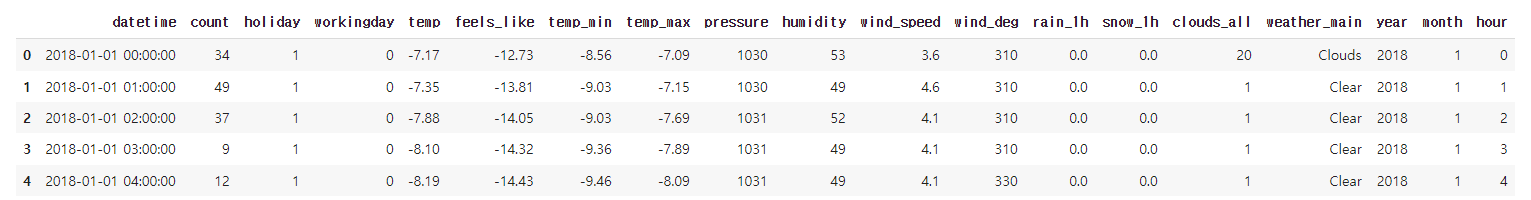
bike_df['year'] = bike_df['datetime'].dt.year
bike_df['month'] = bike_df['datetime'].dt.month
bike_df['hour'] = bike_df['datetime'].dt.hour
bike_df.head()
✔️ 결과
bike_df['date'] = bike_df['datetime'].dt.date
bike_df.head()
✔️ 결과

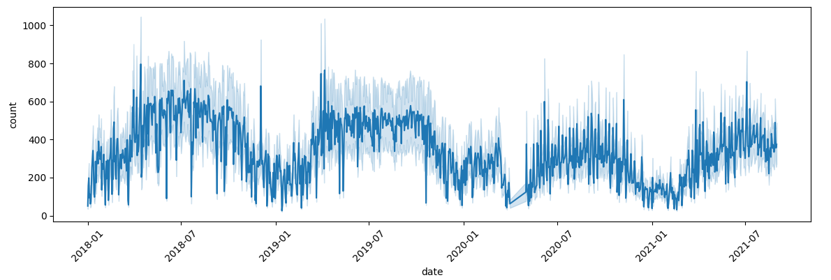
plt.figure(figsize=(14, 4))
sns.lineplot(x='date', y='count', data=bike_df)
plt.xticks(rotation=45)
plt.show()
✔️ 결과
bike_df[bike_df['year'] == 2019].groupby('month')['count'].mean()
✔️ 결과
month
1     193.368862
2     221.857718
3     326.564456
4     482.931694
5     438.027848
6     478.480053
7     472.745785
8     481.267366
9     500.862069
10    446.279070
11    307.295393
12    213.148886
Name: count, dtype: float64
bike_df[bike_df['year'] == 2020].groupby('month')['count'].mean()
# 2020년 4월 데이터가 없음을 알 수 있다
✔️ 결과
month
1     260.445997
2     255.894320
3     217.135241
5     196.581064
6     290.900937
7     299.811688
8     331.528809
9     338.876478
10    293.640777
11    240.507324
12    138.993540
Name: count, dtype: float64
# covid
# 2020-04-01 이전: precovid
# 2021-04-01 이전: covid
# 이후: postcovid
def covid(date):
if str(date) < '2020-04-01':
return 'precovid'
elif str(date) < '2021-04-01':
return 'covid'
else:
return 'postcovid'
covid(bike_df['date'])   # 시리즈를 넣게 되면 하나만 비교가 되기 때문에 결과적으로는 쓸모없다ㅜ
--------------------------------------------------------------------------------------------
#결과
precovid
bike_df['date'].apply(covid)
✔️ 결과
0         precovid
1         precovid
2         precovid
3         precovid
4         precovid
           ...
33374    postcovid
33375    postcovid
33376    postcovid
33377    postcovid
33378    postcovid
Name: date, Length: 33379, dtype: object
bike_df['covid'] = bike_df['date'].apply(lambda date: 'precovid' if str(date) < '2020-04-01' else 'covid' if str(date)< '2021-04-01' else 'postcovid')
bike_df.head()✔️ 결과
# season
# 3~5월: spring
# 6~8월: summer
# 9~11월: fall
# 12~2월: winter
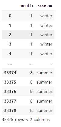
bike_df['season'] = bike_df['month'].apply(lambda x: 'winter' if x == 12 else 'fall' if x >= 9 else 'summer' if x >= 6 else 'spring' if x >= 3 else 'winter')
bike_df[['month', 'season']]
✔️ 결과
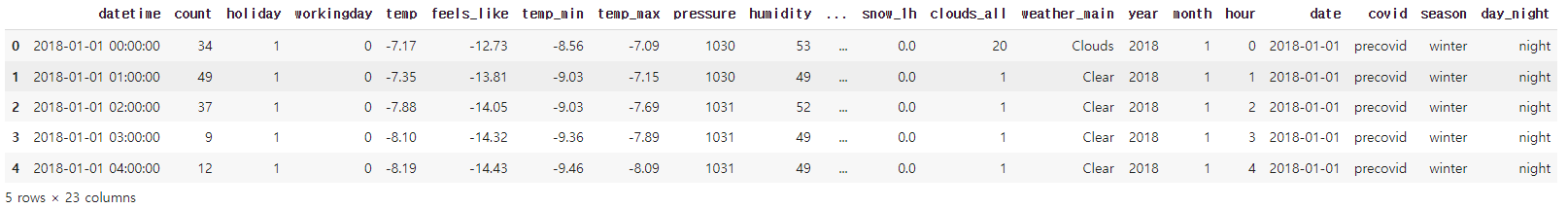
bike_df['day_night'] = bike_df['hour'].apply(lambda x: 'night' if x >= 21 else 'late evening' if x >= 19 else 'early evening' if x >= 17 else 'late afternoon' if x >= 16 else 'early afternoon' if x >= 13 else 'late morning' if x >= 11 else 'early morning' if x >= 5 else 'night')bike_df.head()
✔️ 결과
# 필요 없는 부분 날리기
bike_df.drop(['datetime', 'month', 'date', 'hour'], axis = 1, inplace=True)
bike_df.head()✔️ 결과

bike_df.info()<class 'pandas.core.frame.DataFrame'>
RangeIndex: 33379 entries, 0 to 33378
Data columns (total 19 columns):
# Column Non-Null Count Dtype
--- ------ -------------- -----
0 count 33379 non-null int64
1 holiday 33379 non-null int64
2 workingday 33379 non-null int64
3 temp 33379 non-null float64
4 feels_like 33379 non-null float64
5 temp_min 33379 non-null float64
6 temp_max 33379 non-null float64
7 pressure 33379 non-null int64
8 humidity 33379 non-null int64
9 wind_speed 33379 non-null float64
10 wind_deg 33379 non-null int64
11 rain_1h 33379 non-null float64
12 snow_1h 33379 non-null float64
13 clouds_all 33379 non-null int64
14 weather_main 33379 non-null object
15 year 33379 non-null int64
16 covid 33379 non-null object
17 season 33379 non-null object
18 day_night 33379 non-null object
dtypes: float64(7), int64(8), object(4)
memory usage: 4.8+ MB
for i in ['weather_main', 'covid', 'season', 'day_night']:
    print(i, bike_df[i].nunique())
✔️ 결과
weather_main 11
covid 3
season 4
day_night 7
bike_df['weather_main'].unique()
✔️ 결과
array(['Clouds', 'Clear', 'Snow', 'Mist', 'Rain', 'Fog', 'Drizzle',
       'Haze', 'Thunderstorm', 'Smoke', 'Squall'], dtype=object)
plt.figure(figsize=(10, 5))
sns.boxplot(x='weather_main', y='count', data=bike_df)
✔️ 결과

bike_df = pd.get_dummies(bike_df, columns =['weather_main', 'covid', 'season', 'day_night'])
bike_df.head()
✔️결과
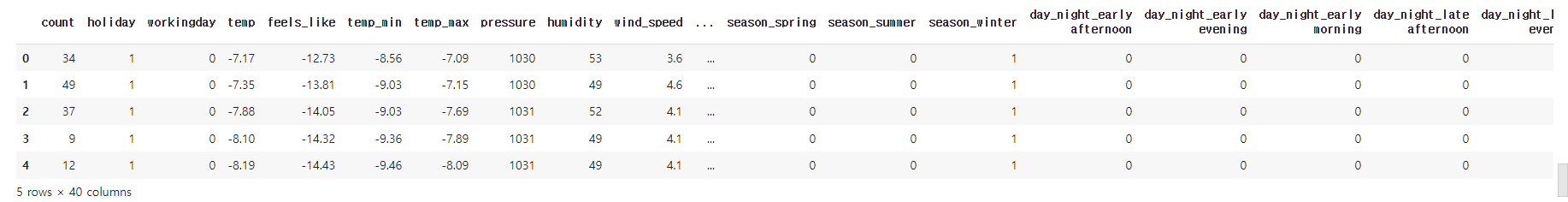
pd.set_option('display.max_columns', 45)
bike_df.head()
✔️ 결과
from sklearn.model_selection import train_test_split
X_train, X_test, y_train, y_test = train_test_split(bike_df.drop('count', axis=1), bike_df['count'], test_size=0.2, random_state=10)
2. 의사 결정 나무 (Decision Tree)
- 데이터를 분석하여 그 사이에 존재하는 패턴을 예측 가능한 규칙들의 조합으로 나타내며, 그 모양이 '나무'와 같다고 해서 의사 결정 나무라고 부름
- 분류(Classification)과 회귀(Regression)모두 가능
- 지니계수(Gini Index): 0에 가까울수록 클래스에 속한 불순도가 낮음
- 엔트로피(Entropy): 결정을 내릴만한 충분한 정보가 데이터에 없다고 보는것. (0에 가까울 수록 결정을 내릴만한 충분한 정보가 있다)
- 오버피팅(과적합): 훈련데이터에서는 정확하나 테스트데이터에서는 성과가 나쁜 현상을 말한. 훈련데이터가 적거나 노이즈가 있을 떄 또는 알고리즘 자체가 나쁠 때 발생. 의사결정 나무에서는 나무의 가지가 너무 많거나 크기가 클 때 발생
- 의사결정 나무에서 오버피팅을 피하는 방법
- 사전 가지치기: 나무가 다 자라기 전에 알고리즘을 멈추는 방법
- 사후 가지치기: 의사결정 나무를 끝까지 돌린 후 밑에서부터 가지를 쳐 나가는 방법
- 의사결정 나무에서 오버피팅을 피하는 방법
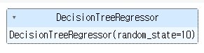
from sklearn.tree import DecisionTreeRegressor
dt = DecisionTreeRegressor(random_state=10)
dt.fit(X_train, y_train)
✔️ 결과
pred1= dt.predict(X_test)
sns.scatterplot(x=y_test, y=pred1)
✔️ 결과
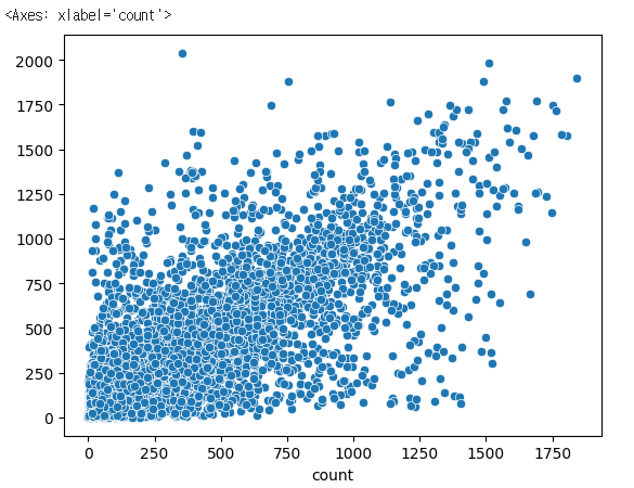
from sklearn.metrics import mean_squared_error
mean_squared_error(y_test, pred1, squared=False)
✔️ 결과
228.428433281008843. 선형 회귀 vs 의사결정나무
from sklearn.linear_model import LinearRegression
lr = LinearRegression()
lr.fit(X_train, y_train)
✔️ 결과

pred2 = lr.predict(X_test)
sns.scatterplot(x=y_test, y=pred2)
✔️ 결과
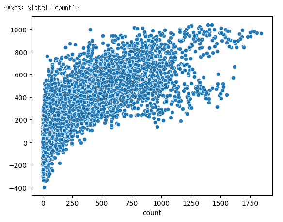
mean_squared_error(y_test, pred2, squared=False)
✔️ 결과
228.26128192004947# 하이퍼 파라미터 적용
df = DecisionTreeRegressor(random_state=10, max_depth=50, min_samples_leaf=30)
dt.fit(X_train, y_train)
✔️ 결과

pred3 = dt.predict(X_test)
mean_squared_error(y_test, pred3, squared=False)
✔️ 결과
228.42843328100884# 의사 결정 나무 RMSE: 228.42843328100884
# 선형 회귀 RMSE: 228.26128192004947
# 의사 결정 나무 파라미터 튜닝 RMSE:
from sklearn.tree import plot_tree
plt.figure(figsize=(24, 12))
plot_tree(dt, max_depth=5, fontsize=12)
plt.show()
✔️ 결과

728x90
반응형